Category Archives: Software Development

Planetary Orbits in Javascript

I have developed an enthusiasm (aka weird obsession) for celestial mechanics and developed several games and the Unity Asset Gravity Engine . In developing Gravity Engine I learned a great deal about high pedigree N-body simulations, but in some cases (e.g. a model of the solar system) it is not really necessary to simulate the system but rather just evolve it in the correct way. In this case Gravity Engine offers the option to use Kepler’s equation and move bodies in their elliptical orbit as a function of time. This uses far less CPU than doing the 9*8 mutual gravitational interactions (10*9, if you add in the “dwarf planet” Pluto).

[If you don’t see an animation, click the post title to see ONLY this post. There is WordPress JS bug when this animation and a YouTube link are present]

Creating code to move a planet in an elliptical orbit with the correct velocity is surprisingly tricky. This is one of those cases where you might expect you could just grab a formula from Wikipedia and bang out some code. This bias comes from all the examples in physics class where the goal is to “find/derive the formula” and get a tidy equation.

If you dig around on physics pages for an equation of an elliptical orbit you will generally encounter the equation for the shape of the orbit with eccentricity e, and semi-major axis, a:

r = \frac{a(1-e^2)}{1+\cos \theta_F}

I have attached the subscript F to the angle to indicate this is the angle from the focus of the ellipse between the position of the body and the long axis of the ellipse. Historically, this angle is named the True Anomaly.

Where is time in this equation?

Nowhere. This equation doesn’t tell us anything about time.

To get an equation for how the object moves as a function of time, we’ll need Kepler’s equation.  Kepler constructed his equation without Calculus (which came along about 60 years after Kepler did this work) using geometric arguments and the assumption that an objects speed in an elliptical orbit was inversely proportional to it’s distance from the focus. Kepler’s equation is:

M = E - e \sin E

Here M is the position of a body moving in a uniform circle at a constant rate (that we will relate to time) and E is the angle to the position on the ellipse from the origin, called the eccentric anomaly. Here a picture will help:

Eccentric_and_True

The eccentric anomaly E is NOT the same angle as \theta_F (f in the picture) however they can be related with a bit of geometry:

\cos \theta_F = \frac{\cos E - e}{1 - e \cos E}

\sin \theta_F = \frac{\sqrt{1-e^e} \sin E}{1 - e \cos E}.

If we have a specific time we want a position for we need to convert this into a value of M. This is done by dividing the time by the time per orbit, T. Kepler can also help us here with his third law that relates the size and eccentricity of the orbit to the mass of the bodies:

T = \frac{\sqrt{a^3}}{m}

where m is the combined mass of the central object and orbiting body. (Kepler did not know the proportionality constant was the mass, that came later).

Given M, Solve for E

Ok, we’ll just isolate E…hmmm. E appears by itself and inside the sine function. That sinks our chance of getting a tidy mathematical formula. This equation is legendary in Mathematics, since it is an early example of a transcendental equation with an import application. It has been studied extensively and the approaches are well summarized in the book “Solving Kepler’s Equation Over Three Centuries” by Peter Colwell.

There are some series approximations, but they are not valid for all eccentricities. The most common approach is to iterate the equation until we converge on a value that is “good enough”.

The “recipe” for tying this all together is:

  1. Determine the orbital period T
  2. For the time t we’re interested in, divide by the orbital period and use the remainder to find the angle if the body were moving in a uniform circle, M.
  3. Using iteration solve Kepler’s equation and find E
  4. Using E, determine \theta_F
  5. Find the corresponding r using the orbit equation.

In Javascript this becomes:

var orbitPeriod = 2.0 * Math.PI * Math.sqrt(a*a*a/(m*m)); // G=1

function orbitBody() {

 // hide last position drawn
 context.clearRect( last_x -10, last_y - 10, 20, 20);

 // 1) find the relative time in the orbit and convert to Radians
 var M = 2.0 * Math.PI * time/orbitPeriod;

 // 2) Seed with mean anomaly and solve Kepler's eqn for E
 var u = M; // seed with mean anomoly
 var u_next = 0;
 var loopCount = 0;
 // iterate until within 10-6
 while(loopCount++ < LOOP_LIMIT) {
 // this should always converge in a small number of iterations - but be paranoid
 u_next = u + (M - (u - e * Math.sin(u)))/(1 - e * Math.cos(u));
 if (Math.abs(u_next - u) < 1E-6)
 break;
 u = u_next;
 }

 // 2) eccentric anomoly is angle from center of ellipse, not focus (where centerObject is). Convert
 // to true anomoly, f - the angle measured from the focus. (see Fig 3.2 in Gravity) 
 var cos_f = (Math.cos(u) - e)/(1 - e * Math.cos(u));
 var sin_f = (Math.sqrt(1 - e*e) * Math.sin (u))/(1 - e * Math.cos(u));
 var r = a * (1 - e*e)/(1 + e * cos_f);

 time = time + 1;
 // animate
 last_x = focus_x + r*cos_f;
 last_y = focus_y + r*sin_f;
 drawBody( r* cos_f, r*sin_f, "blue");
 setTimeout(orbitBody, 30);
}

I have left out some of the init code for clarity. If you view the source for this page you can find all this.

(Eccentric anomaly image created by CheCheDaWaff/Creative Commons License).
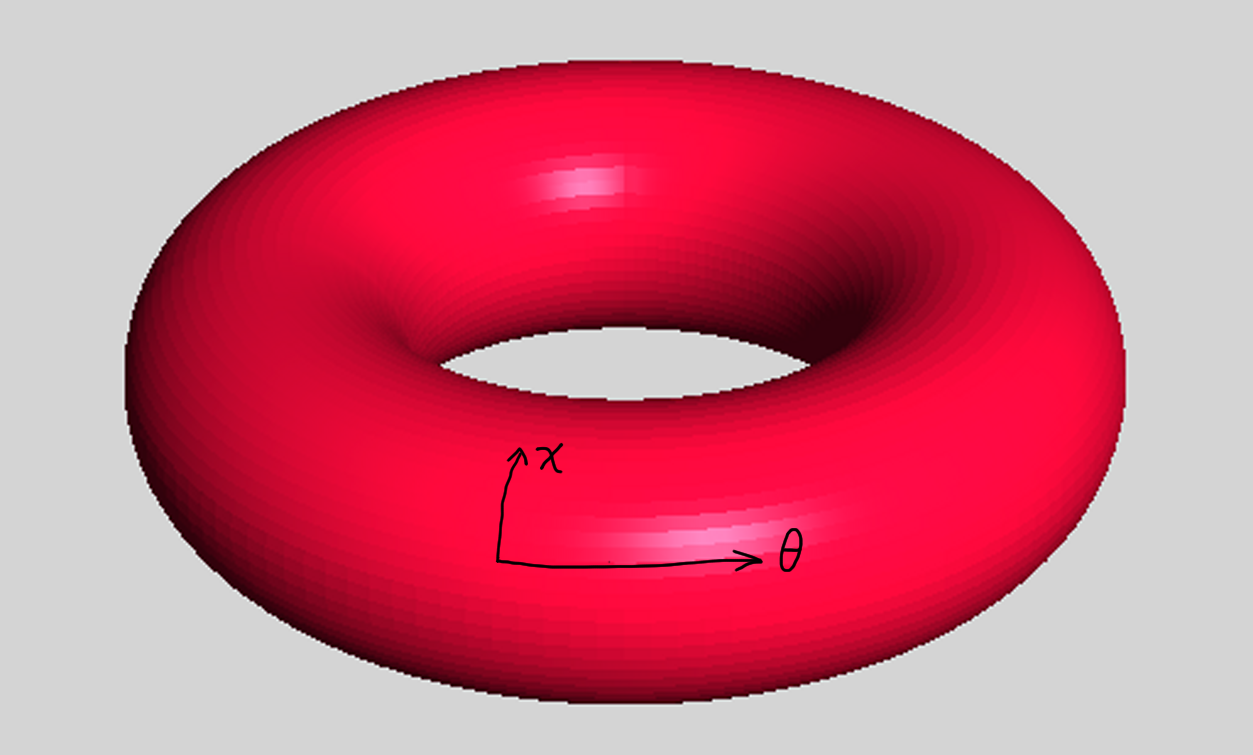
Asteroids on a Torus

One of the great things about meetups is their ability to generate weird idea exchanges. Late last year I demonstrated ThreeBody – another of my oddball, limited appeal physics apps. I was mentioning that it might be fun to see what happens to the three body problem in a spherical space – since this would solve the “ejection to infinity” issue by removing infinity. This led to a discussion about the topology of games like asteroids where the top/bottom and left/right are wrapped. This mapping creates a space that is a topological torus. This was the spark I needed to think more carefully about what motion on a real torus would be like.

I don’t need much of an excuse to think about an odd physics scenario.  My past includes time spent taking a break from the working world and doing a PhD involving curved spacetimes. One of the problems that comes up in such studies as a way of sharpening skills is the study of motion on curved 2D surfaces. It is a great place to learn to use the mathematical machinery and intuitive enough that the answers can be visualized.

This made me wonder how different a space shooter would be if the physics of a torus was made “technically correct” (the best kind of correct) . The result is a soon to be released game “Geodesic Asteroids” in which there is a dual view of the 3D motion and the 2D motion with the paths of objects moving in a “technically correct way”.

 The Torus

Torus1

Figure 1: Torus coordinates

First we need a mathematical description of the torus. It is a 2D surface so only two co-ordinates (\theta, \chi) are needed to describe a point. If we think of the typical donut representation sitting on the x, y plane then \theta is the angle around the z-axis (say from the line x=0) and \chi is the angle around the cross section of the torus at a given \theta. The radius of the center of the torus is a and the radius of the cross section is b.

In the mathematics for a torus, everything can be described in terms of these co-ordinates, including the equations of motion that define how an object moves when there is no force on it. We are accustomed to thinking of the torus as a three dimensional object but exactly which three dimensional shape results is partly due to the choice made when we embed the surface in 3D. There is really no reason we have to do this but it can help our intuition. [Digression: It an interesting mathematical question about exactly how may dimension are required to embed an N dimensional surface, we are accustomed to N+1 for e.g. spheres and torii but this is not the general rule!].

In our case we pick a customary embedding:

$$x = (a + b \cos{\chi}) \cos{\theta}$$

$$y = (a + b \cos{\chi}) \sin{\theta} $$

$$z = b \sin{\chi} $$

This allows us to map (\theta, \chi) into the x, y, z world co-ordinates the game will use and retain our intuitive picture of a torus.

What about a 2D map of this torus? Here I elected to just use (\theta, \chi) as pure 2D co-ordinates i.e. as if they were the displays “x and y”. I impose a slight twist that I’ll explain in a minute.

Motion on the torus

The embedding equation provides the world space position to show events on the torus. What equations should be used to calculate motion on the torus? The motion takes place on the torus so the description is in terms of  (\theta, \chi). Here there is a departure from the usual equations that govern games. In the flat 3D game world x, y and z are independent and there is no need to worry about where in the space we are. F=ma is the same at the origin as it is at any other point. On curved surfaces things are different. To make this clear lets consider a simpler 2D surface, the sphere, with longitude \phi and latitude \theta.

greatCircle

As you know from looking at maps of airplane flights, the lines between points take what seem to be curves on the map. This is because the force-free (or geodesic) path that connects two points is a great circle. This means if you are in New York and head directly west the geodesic path must be a diameter of the circle and will carry you into the southern hemisphere until you are at the antipodal point directly opposite New York through the center of the earth. [Fun fact: very few places on land have an antipodal point on land]. You started out with only a velocity in the \phi direction but ended up on a trajectory for which \theta also changed. This means that the equations of motion are coupled. The equation for the evolution of \theta depends on the velocity in the \phi direction. In the case of a sphere the equations for force free motion are:

$$a_{\theta} =v_{\phi} v_{\phi} \sin{\theta} \cos{\theta} ,  a_{\phi} = \frac{-2 v_{\theta} v_{\phi}}{\tan{\theta}} $$

For a torus the equations are:

$$a_{\theta} = \frac{2 \sin{\chi} v_{\chi} v_{\theta}}{b (a + b \cos{\chi})}, a_{\chi} = – \frac{2 \sin{\chi} v_{\theta}^2}{(a + b \cos{\chi})} $$

The good news is that on the torus the co-ordinates are well behaved. The expression are finite. (If you look at the equations for the sphere you’ll see it is possible for some values to be dividing by zero. Never a great idea. This is not a fundamental part of motion on a sphere, there is no special place where acceleration goes to infinity. It’s just a bad choice of co-ordinates and we need to choose a different origin in some case. It is quite usual to have to cover a surface with several co-ordinate patches. For the torus we are lucky that this is not needed.)

Where did those equations come from?

The equations for F = m a 
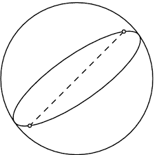
on a curved surface come from a branch of mathematics known as differential geometry. “Differential” since it studies the behaviour of surfaces that are smooth enough that you can do calculus, i.e. no sudden steps or cusps. One of the new ideas that enters with differential geometry is that while you can do calculus at each point, you cannot directly compare the results of these calculations at different points. This is because each point has its own tangent plane (more generally tangent space). As an object slides along the 2D surface the local co-ordinates of the object change relative to the surface co-ordinates. Returning to our sphere example, if you initially were heading west from New York when your great circle crosses the equator you are no longer facing west BUT you did not turn, you were just following your geodesic path. Exactly what the geodesic path is and how it turns as you go is something that can be calculated for a surface.

It’s not my goal to turn this post into a treatise on differential geometry. It is a very interesting subject and is the stage on which Einstein’s General Theory of Relativity takes place. All the introductory GR texts start with some background in differential geometry and I find their approach more geared to my interest than the way math books approach the subject. For those interested in a good introduction to the geodesics of the torus and an introduction to the basics of differential geometry, I recommend Jantzen’s paper. My favourite intro GR book is Schutz’s “A First Course in General Relativity”

Differences between 2D and 3D representations

A space game on a torus can be shown in 3D but it is also interesting to play the game on the 2D representation of the surface. Here the odd paths of the objects make the impact of the curved surface apparent. There are some compromises in mathematical purity that I have made in the interests of actually finishing the game. The primary one is that the size of objects in the 2D and 3D view cannot be fully reconciled (more below).

On the true mathematical surface the distance travelled as you walk around the outside diameter is different from the inside diameter. On the 2D map this means that the top edge of the map should not be as wide as the middle. Our choice of a 2D map is therefore vulnerable to the an effect similar to that occurring on a Mercator projection of the Earth (Greenland is shown as far too big).  I have chosen a simple scaling depending on the “latitude” \chi. To continue this accuracy it is necessary to change the horizontal size of the objects as they change latitude. I did put this in the game as an option – but the result is a bit odd looking. In normal play this mode is disabled – with the consequence that the objects on the screen are not exactly the correct size. The correct size is used for detecting bullet hits and in some cases an apparent hit on the map is not a “real” hit.


True scaling leads to some weird paths in the map view. If an object is moving quickly in \chi the shrinking due to the scale factor can exceed motion towards the edge making it look as if the object backs up a bit before continuing on.

Geodesic Asteroids is available on Blackberry, iOS and Android. It has been great fun to think about and use the geodesic math I learned long ago. It is also the first time I have written a more “video game” style game. Hope you’ll find it interesting.

[social4i size=”large” align=”float-right”]

iOS: A Three Year App Development Odyssey

I have spent three years of spare time to create a single App. Upon reflection this seems more than a little crazy until I remind myself that the goal was not so much to get the App out into the world but to teach myself about iOS game development from “soup to nuts”. It was very satisfying to be completely curiosity driven.  This was a complete departure from the ruthless pragmatism that informs the way I code in my day job.

The catalyst was the fact that in my day job I had taken on the role of leading R&D in a start-up. The dev team knew what they were doing and what the company really needed me to do was articulate our vision to customers and analysts. As a result I found I had traded in Eclipse for Powerpoint and Word. After a while I found that I really missed the kind of problem solving that comes with developing software. At the time iOS was really hot and a hobby project in this area seemed like a good idea (admittedly, not an original thought).

When I get a blank sheet of paper I generally do something relating to physics. I had the great fortune to evolve from an undergrad in engineering into graduate degrees in physics. I had nearly gone into physics instead of engineering as an undergrad but I was wisely counselled that engineering had a much better chance of paying the bills – unless I was sure I could be at the top of the class. Good advice – and apart from a sojourn in graduate school my software skills have been how I pay the bills. When Java first came out, during my PhD in general relativity, I created applets that showed orbits in a variety of different forces. It seemed natural to try and link iOS and gravity in some way.

The journey started with something not too different from the old Java code from long ago. I got some basic iPhone code running with Quartz graphics added a bit of touch interaction and simple gravity evolution. It was ok but seemed a bit uninspired. At the time there were people in the startup doing graphics stuff. They kept talking about shaders and GPU code and I was curious about their world. I also thought it would be cool to make the gravity simulation do proper 3D. At this point I probably had invested about five months in iOS to get the Quartz game going. I decided to press reset and start again in OpenGL.

Getting OpenGL up and running was a BIG deal and caused at least a six month hit. It takes a while to have the right mental model of what is really going on in the shaders and without a graphics debugger using only newbie knowledge I ended up doing a huge amount of experimenting. The resource I used at the time was a book iPhone 3D Programming. This was a good introduction to OpenGL ES and I went between it and the Blue Book. I was able to get some reasonable 3D stuff going. I did find the C++ cross-platform framework in the iPhone book a bit unsatisfying. After all I was also trying to get some chops in Objective-C. However, I had running code and started to work on the touch interface and game flow.

During this time, in my day job, I had realized I just did not have the temperament to pitch for a startup and wave the flag day after day. I found a senior software role in a mature company and started to wade through their code. It is hard to adequately convey how bad this code was. As a consequence I started to read about dealing with bad code and started to take Clean Code seriously. This had repercussions in N-body. Since I could not have clean code “at the office” I tried extra hard to keep N-body clean. This resulted in some significant refactoring in N-body.

Then iOS5 came out. It had GLKit routines for math and utility routines for texture loading at a time when I was just starting to realize the values of texture atlases. Again, I rushed towards the shinny new thing and refactored out all the C++ code making some structural improvements along the way. I found it very useful to revisit design patterns in the context of Objective-C. The structure of a language and it’s libraries often informs the style in which common problems get solved. I found Cocoa Design Patterns a big help in getting into the flow of Objective-C coding. Another big bonus was a colleague who had a long history in MacOS development and was generous with his time. I also used this opportunity to go all the way to the bottom in OpenGL. Since I had no strict self-imposed deadline I messed around with how vertices were generated, how the lighting in the shaders work, normal maps for texture simulation, how to map strings into textures into transparent objects, and on and on. (Once iOS6 came along the Xcode OpenGL debugging became much easier. That feature in Xcode is hugely powerful).

In parallel with this I was working through Solar System Dynamics and became entranced with the weird tadpole and horseshoe orbits that occur as bodies oscillate about Lagrange points. I really wanted to show these orbits in the co-rotating frame and find a way to interactively generate some intuition about how variations in starting conditions affect the orbit. This added more time to the development. Then I stumbled into the choreography orbits. These were amazing but didn’t quite hang in there with the integrator I had in my physics engine. This sent me on a detour to learn more about choreographies and change the physics engine to do fourth-order Runge-Kutta evolution.

Finally, it seemed like a good idea to have built-in autoplay for all the levels – so I could regress after making changes to the integrator. This took a further investment in time but one which on reflection was time well spent. I found a number of issues during these regression tests.

Then it was time to polish. This is a challenge for me. I have a half dozen other cool physics game ideas and a shelf of unread books. Somehow I managed to stay focused and get N-body done to a level that I felt I could stand behind. There are things I wish were better, levels I wished I had time to add but I forced myself to just record all the diversionary ideas and after two and half years stop wandering off and stop the feature creep.

Finally, I started beta testing (using TestFlightApp as recommended by a friend – it’s awesome). Bugs were found, discussion on the merits of what the app was and wasn’t were had. After some reworking and a bunch more polish I deemed it was ready to submit.

Okay, I think I get where the three years went.

Hunting Zebras in Outer Space

I once took a graduate course: ”Physiology of Excitable Cells I” run by an eccentric British professor who wanted to teach in a far-reaching classical sense. (In the first class on hearing my surname he commanded ”Next week you will tell the class the connection between your name and Sherlock Holmes”; perhaps a bit off-topic given the course title). One thing he said that has stayed with me is that common problems have common solutions. He was discussing how all the medical students he taught were quick to assume a patient had a rare condition, instead of something more mundane. The tag line they teach medical students is:

“When you hear the sound of hooves, think of horses not zebras”.

I use this phrase a lot when it comes to debugging issues in software. It’s far too easy to believe I am the victim of some fiendishly clever interaction in my system or (so help me) a compiler bug. The answer is (to first order) always that I have done something very dumb or just failed to see an edge case. After a long time writing code I am a lot less likely to get caught by this. However, it did happen to me with N-Body and I was so amazed at how dumb I had been I had to close the laptop and go for walk.

The issue related to the use of sprites for a collision. They seemed to work pretty well except on a level where I had a number of other masses moving around. The latent trap was that I felt guilty about the quick way I had pushed sprites into the code. I decided not to worry too much about optimizing them and allocated a sprite group on the fly. I know it’s better to pre-allocate a sprite pool and all that – but at the time I added them my main focus was elsewhere and I knew I would have to come back and clean them up.

So when I hit an issue where collisions on a busy level resulted in a serious pause in the game loop – I decided the time had come to finally put in sprite pools. That HAD to be the source of the issue. Off I went, with the added fun of feature creep in the refactoring. All in all I spent about ten hours. It made no difference.

The real issue showed itself when I was doing the feature creep part of the refactoring. The loop nesting was wrong and I was running the sprite evolution inside a loop that was running over each body in a level. When there were five masses, I evolved the sprites five times per clock tick and things got really slow. Instead of looking hard for a simple error I had jumped to the conclusion that it must be due memory inefficiency and my use of on-the-fly allocations. Doh! I was amazed I had gone on such a long Zebra hunt.

I have used the Zebra hunting metaphor for such a long time that sometimes I now use it without setting the context properly. I was working with our very bright overseas team in India but thought that this time they were on the wrong track, chasing a theory that seemed too intricate. When my manager asked me how they were making out I responded ”Oh, I think they’re off Zebra hunting”. He replied ”Really?! Do they have a holiday or something?”. I then explained my metaphor as well as the fact that India does not have Zebras…