Two New Celestial Mechanics Books + Another One

Even though I already have a sizable collection of books on orbital mechanics I cannot
resist adding more. Recently two new books came to my attention and inevitably the references in one of them led me to a third book. Here is a brief overview based on a “reading” (i.e. not studying in depth) of the first two and a browse through of the third.

They are very different in approach and scope and both very worthwhile.

Moving Planets Around

Moving Planets Around: An Introduction to N-Body Simulations Applied to Exoplanetary Systems

Moving Planets Around is a fantastic resource to get started with N-body gravitational simulations. It is strongly motivated by the on-line book by Hut and Makino “Moving Stars Around” circa 2003. Hut and Makino has a warm place in my heart since it was one of the key resources I used when creating the original N-body code that led to Gravity Engine.

Moving Planets Around begins with the same premise of building an N-body simulator from scratch and builds up to a modern scenario of examining the stability of moons in exoplanet systems. It starts at a very basic level and goes from Newton’s gravity and the two body problem into three body dynamics. As is appropriate for this subject is also spends a significant amount of time on the details of how to evolve these equations numerically, covering the essential numerical techniques used in this field.

All of this is done in a literally conversational tone. The book is written as a dialog between two graduate students Alice and Bob working on a project from scratch with the assistance of Professor Starmover. At first this is a bit distracting but it has some advantages in that it allows some “wrong-turns” to be brought forward and discussed in a very natural manner. This dialog approach was one of the key features of “Moving Stars Around”.

If you have any interest in the issues that come into play when doing numerical modelling of small planetary systems, this is an exceptionally approachable book. All the code examples are in Python and an accompanying GIT project provides them all on line. The code is GPL, so while I find it useful as a source of ideas I have not downloaded it or made use of it in my Gravity Engine project.

Dynamics of Planetary Systems

Dynamics of Planetary Systems (Princeton Series in Astrophysics) by [Scott Tremaine]

The other VERY new book I have read the first half of is “Dynamics of Planetary Systems” by Scott Tremiane (emeritus professor at the Institute for Advanced Study). When I saw this book as a pre-order on the Princeton University Press website I immediately ordered it. Tremaine is a giant in the field and with Binney wrote “the book” an the motion of stars in galaxies “Galactic Dynamics”. I was not disappointed.

The book is ultra-modern and pragmatic in it’s view-point. Tremaine points out that many of the earlier treatments of planetary systems involved long and tedious treatments of how planetary orbits are perturbed by other planets and in the modern age this is either done with computer algebra or numerical modelling. [I can attest to the length of these calculations, having done them as exercises at one point.]

Whereas “Moving Planets Around” is a very friendly introduction for the novice, “Dynamics of Planetary Systems” is an amazing resource for a graduate student or senior undergrad in physics. It covers the basics of orbits as a warm up and then gets into the real fun of three body systems and beyond.

The nuggets of wisdom I have tagged for further study include:

  • the gold standard for planetary dynamics simulations is REBOUND [LINK] (again GPL, so nothing I wish to download)
  • there is no “one size fits all” numerical integration algorithm. The choice depends on the number of bodies and the timescale required. There are special purpose techniques when interested in the long term stability of the solar system.
  • spin-orbit resonances and tides are very cool. I *really* need to spend some time with these chapters!

Celestial Mechanics and Astrodynamics: Theory and Practice

Celestial Mechanics and Astrodynamics: Theory and Practice (Astrophysics and Space Science Library Book 436) by [Pini Gurfil, P. Kenneth Seidelmann]

This book was referenced in “Moving Planets Around”. The title caught my attention since all the other books on my bookshelf have title that mentions either celestial mechanics or astrodynamics, so a title that mentions both is immediately interesting to me.

First the book is a bit pricy. My book collection “bug” means I am on the mailing list for many of the technical book providers and Springer, in particular, has occasional amazing sales (in the 40-50% range). There is usually a 50% off sale around Christmas, and nothing says Christmas more than a shiny blue graduate-level physics book! In the case of this book I was able to get 40% off.

Ok, the book.

First, it covers a lot of material. Some of this is in enough depth to be all you need and in other cases its purpose is to make you aware of a field. For example when discussing stability of orbits it has a brief discussion on Poincarre sections that is largely a pointer to other work.

There are some things described in detail here that I have not seen elsewhere in my orbital mechanics library. There is a derivation of Hohmann transfers in the presence of a J2 term that describes the gravity of an oblate planet. That’s pretty cool. There is also an excellent chapter on motion around oblate planets, which is something I need to go back and study.

While I need to spend more time with this book, I regard it as a worthwhile addition to my bookshelf.

In Closing

I’ve enjoyed welcoming these books to the shelf and there is value in each of them. They’re a good distraction as I undertake the re-writing of Gravity Engine. Seven years after the initial version I now know much more about orbital mechanics and am looking forward to developing a much more streamlined Unity asset that will allow growth into more complex gravitational problems.

Equal Spacing Around an Ellipse

My Unity asset Gravity Engine models orbits around planets. These are typically ellipses so gravity engine generates a lot of ellipses. The simplest way to do this is to use an equation for the ellipse in polar coordinates and take equal angle steps in the angle and link the points together. These points are then used by a line renderer to make the ellipse. As the ellipse gets more elongated there are issues at the ends and it starts to look “janky”.

The ideal would be to create points that were equally spaced along the ellipse. How hard could that be?

Pretty hard, actually.

This is one of those interesting math puzzles that gets under my skin. What is especially interesting about this puzzle is that it is not a bunch of messy algebra (in fact the equations end up being quite simple), it’s that the equation that results is an integral that does not have a tidy solution. The integral is common enough that the way this gets handled is that a new function is defined as the solution to this integral. In this case events hinge around finding a solution to the integral:

 E(\phi, k) = \int_0^{\phi} \sqrt{1-k^2 \sin{\theta}^2} d\theta

In fact, just to increase the “fun factor” this equation needs to be solved for a specific length around the ellipse i.e. for a given value of E(\phi, k) = s find the value of phi (which is in the limit of the integral).

I have written up the details of this in a white-paper on this site. This allows me to write up the topic in more detail and to provide a better format for reading the equations than this blog allows. It also spares people from the gory details if they do not want to see them.

I implemented the full-on numerical solution using elliptic functions in the latest version of the Numerical Tools asset. I also show a much simpler heuristic in which the steps in angle are scaled by (r/a)^{2/3}. The comparison of these is shown below.
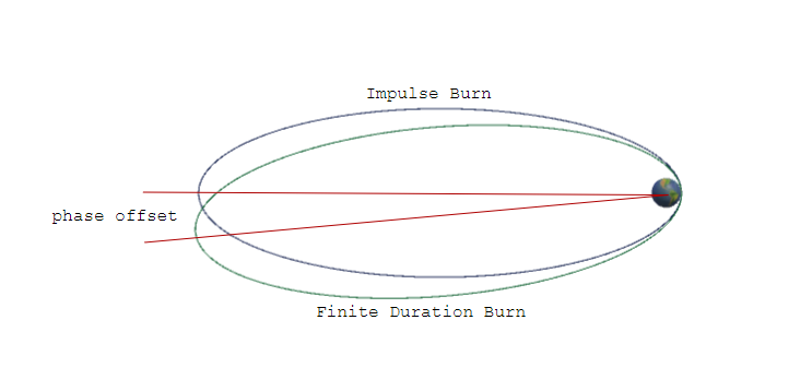
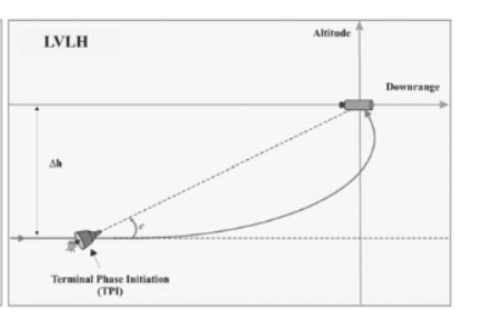
Exact equal spacing (red squares) versus simple heuristic (blue dots).

Which Direction to Burn? Finite Burn Hohmann Transfers

A Hohmann transfer calculation changes the circular orbit of a spacecraft using an impulse burn along the prograde direction of the initial orbit. Real spacecraft burns take time, e.g. the Apollo transfer to the moon requires a burn of about 350 seconds. I was recently asked by a developer using Gravity Engine about how the spacecraft should steer during this burn time. Should it keep the initial attitude when the burn started? Burn “forward”? Burn perpendicular to the Earth radius vector? Great question! (The question comes from the developer of ReEntry, a must have if you’re a vintage space buff!)

In the interests of not re-inventing the wheel and limiting the amount of “rocket science” I do, l first turned to my bookshelf, Google and the literature. Unsurprisingly, this is a “whole thing”. Since the trajectories of missions are planned using highly detailed iterative simulations coupled with optimal control theory the literature is highly technical and not something I can easily map into Gravity Engine. Instead I decided I would do some basic experiments with three steering laws:

  1. Lock on to the initial burn direction and maintain it.
  2. Burn in the “forward” direction
  3. Burn perpendicular to the Earth orbit radius in the orbital plane

In addition to direction, there is an issue of timing. If the burn will be on the order of 350 seconds, where should the burn start with respect to the desired destination point? Instead of varying this as an input parameter, I elected to measure the result when arriving at the destination: how far away from the point opposite where the burn started did the ship reach the destination orbit?

It’s always fun to think about the physics here and try and guess which steering mode will give the most efficient transfer. My guess was that by thrusting perpendicular the maximum amount of angular momentum would be added and this approach would use the least fuel. I then build a scene in Gravity Engine to assess these choices.

Gravity Engine allows a direct Hohmann transfer to be computed via its TransferShip component. This is used to provide a reference transfer. Since the scenario I was asked about was related to Apollo, I used some approximate values for ship, stage and fuel mass and used a rocket engine model that accounted for the decrease in mass as the ship burned fuel. I then created a FiniteBurn component to run the steering algorithm. I have archived this demonstration code for interested users of GE.

The results are:

ModeActual Burn TimePhase Offset
SIVB EngineTangent299.611.03
Perpendicular299.7912.52
Fixed3034.79

Three things about this are interesting:

  1. The total burn time to reach an apogee at the Moon’s distance is not very strongly affected by the choice of steering law.
  2. The angle offset of the arrival point is strongly affected by the choice. The timing of when to start the burn DOES depend strongly on the steering law.

It’s a good thing I do experiments instead of trusting my intuition. Thrusting perpendicular to the radius was not the most efficient steering law.

Point and Burn

The thing I love about having diverse customers for Gravity Engine is that the questions they raise force me to extend my knowledge of orbital mechanics beyond the “simple” treatments presented in the textbooks. Recently, the developer of the very impressive ReEntry game highlighted the fact that the Hohmann and Lambert rendezvous code in Gravity Engine was cool, but it did not match the method used by NASA for Gemini and Apollo rendezvous. NASA used a maneuver called trigger angle targeting that used a burn in the line of sight direction from the ship to the target. Ok, I thought, time to dig through my 12 orbital mechanics books and see what’s up with this. Only two of the books mentioned this mode of rendezvous. Walter’s Astrodynamics mentions this in an informational box on NASA rendezvous techniques and provides some references. Practical Astrodynamics by de laco Veris presents an iterative solution.

Trigger angle maneuver (Figure from Woffinden, Rose and Geller, link below)

First a bit of background on this technique in the context of Apollo lunar rendezvous. This rendezvous mode is used in the final phase of rendezvous when the LM and CM are already in circular coplanar orbits with a modest difference in radius (e.g. 28 km). The LM catches up from below and behind and when the CSM is at a specific angle above the horizon (about 27 degrees) it burns directly towards the CSM. This has the advantage of allowing a manual orientation and burn in the event of computer issues or loss of communication. Point the ship at the target and burn. The burn magnitude is based on a calculation that factors in the desired time to rendezvous. In the Apollo case the time to rendezvous was chosen such that the CSM moved through about 130 degrees of it’s orbit.

I first considered the usual rendezvous approaches to see how they compared. A Hohmann transfer requires the CSM to move through 180 degrees and has a burn direction parallel to the local horizon. It is the most efficient transfer but the ship needs to be pointed towards the horizon. A Lambert transfer to the desired rendezvous point could be done but the velocity vector is unconstrained and in general will not be in the direction of the CSM. Quantitatively how do these compare to the actual Apollo 11 burn?

TypeAngle from Horizon (deg)Burn Magnitude (m/s)
Hohmann06.62
Lambert20.977.83
Trigger Angle25.548.24

Note that the trigger angle is a more expensive option in terms of dV. The fault tolerant procedure comes at a cost. Neither the Hohmann or Lambert transfer is providing the trigger angle burn needed for Apollo 11. Gravity Engine clearly needs some new code.

The trail starts with a paper from 2007 by Woffinden, Rose and Geller that demonstrates how to solve for a trigger angle given that the burn must be in the direction of the target. I found it a bit surprising that this analytic result was published 45 years after trigger angle targeting was used in Gemini! This paper also references the very readable Navigating the Road to Autonomous Orbit Rendezvous by Woffinden and Geller.

The approach taken in the trigger angle paper is to use a local co-rotating co-ordinate system with the rendezvous target at the origin. This system assumes the target is in a circular orbit and the ship is “relatively close” to the target. This system is often referred to an Local Vertical Local Horizontal or LVLH. The rendezvous equations can be mapped into this co-ordinate system with a few simplifying assumptions and the result is the Hill-Clohessy-Wiltshire equations that describe the relative motion of the ship with respect to the fixed target.

The new code added to Gravity Engine provides a RelativeMotion class that provides the Hill-Clohessy-Wiltshire rendezvous equations and an additional module to perform the trigger angle targeting. The result of this code for the Apollo 11 case produces the trigger angle and burn shown in the table above. When used “as is” the resulting rendezvous in the fixed target frame is:

By itself this burn does not result in a perfect rendezvous. After braking the LM is 3.55 km away from the CSM with a residual velocity of 2.9 m/s. Further nuance is needed.

The Apollo 11 terminal phase included two course correction burns and a series of braking maneuvers at fixed distances from the CSM (LM burn schedule). To include this a TPIBurn class has been added to Gravity Engine to handle the sequencing of these events in addition to the initial TPI burn. By adding these elements to the scene the rendezvous now concludes with the LM 21 meters away from the CSM with a negligible residual velocity.

This code will be available in Gravity Engine release 5.0.

“Three is too much things”

Sometimes a web comic speaks to your soul. The title comes from the hover text of this SMBC comic. At the time I was working on my third attempt to create code for a Lunar free-return trajectory and add it to gravity engine. With the release yesterday of Gravity Engine 3.2 there is now a passable effort at this somewhat difficult problem. It was important to me to get something working since several users were keen to include this in their games. The result allows mission planning for a patched conic “on-rails” trajectory that loops around the moon.

The mathematics behind the patched conic approximation is fairly straight-forward. It is often described in textbooks in the context of a mission to another planet.

The free-return problem adds a significant complication since the return path after lunar flyby needs to bring the spacecraft back to Earth and the path needs to impact the atmosphere to ensure re-entry. This adds an additional constraint to the motion that is already constrained by a desired time of flight to the moon and a specific perilune approach target. The scene created for Gravity Engine 3.2 allows this to be explored interactively. Doing this you discover it is a very difficult to meet all three goals and this is the “simplified” version of the problem using patched conics!

This scene is a step in the right direction but I still find it a bit disappointing. I want Gravity Engine to move in the direction of a tool that allows game developers to just “Make It So”. I want a system where the desired free-return attributes are given and the code can do the astro version of “path finding” to make it happen.

Gravity Engine 3.2 is now live on the Unity Asset store. The details of how the free-return scene works are here.

Is Unity Good at Orbits?

As the creator of the Unity asset Gravity Engine I was curious about how well Unity modeled orbits without all my extra work. In investigating the way that Unity is doing physics I came across a very dramatic difference in performance based on the order of two lines of code and a numerical method I should have known about!

A Unity project with these demonstrations can be found on github.

The “natural approach” is to use Unity do the physics  with a rigidbody AddForce() to provide the gravitational interaction. This requires a script with a FixedUpdate() that determines the force of gravity due to some other object based on that objects mass and distance. For simplicity we’ll consider just one “heavy” object in the scene at the origin. The result can be seen below. The trail of the object does not form a closed orbit (as it should for Newtonian gravity) and the orbit axis shifts over time. Does this provide a clue about the way Unity is doing physics?


In order to investigate how Unity is evolving the force (i.e. what numerical approach it is using) we can now create some mini-physics engines of our own and see how they compare to the result from AddForce().

Creating a simple physics integrator for a single body is straight-forward. In a FixedUpdate() method we can update position by a time step, calculate acceleration due to gravity and use it to advance velocity by a time step.

The simplest algorithm (Euler)  updates position and velocity each time step (r, v and a can be Vector3 or this can be taken as pseudo-code for array operations):

// Euler update
r = r + v * dt; 
v = v + a * dt;

In my initial coding, I did this from memory and typed:

// NOT Euler (velocity is updated first)
v = v + a * dt; 
r = r + v * dt;

this is NOT Euler and this make a very big difference!

In addition we’ll compare the simplest of the integrators in Gravity Engine, named LeapFrog (or Verlet depending where you look). It is:

// Leapfrog
v = v + a * 0.5 * dt;

r = r + v * dt;

v = v + a * 0.5 * dt;

Taking a look at these algorithms:

Wow. Euler is terrible; the orbit is not even closed. The “Not Euler” method is pretty good and is quite close to what Unity does. Leapfrog is also pretty good and looks to be about the same as “Not Euler”.

The “Not Euler” method is more correctly called the Semi-Implicit Euler method. The key is that the velocity is advanced to the next time step before it is used. This seems like a weird mix – using the velocity from a time step ahead to update the position in this time step. What surprised me was given how well this works, why it does not come up in the scientific introductions to N-body integration (e.g. Moving Stars Around). I assume they go direct to Leapfrog because they are headed to more complex algorithms and Leapfrog is a useful segue. The Semi-Implicit Euler method shares an attribute with the Leapfrog integrator. They are both good for systems in which energy is conserved, like gravity. Technically they are called symplectic integrators due to the way the preserve area in a phase space of position and velocity. Semi-Implicit Euler is the simplest symplectic integrator, Leapfrog/Verlet is a second order symplectic integrator.

What is AddForce() doing?

It appears that Unity AddForce() is keeping up well with Semi-Implicit Euler and Leapfrog.

Can we figure out which one it is using?

Let’s take a look at how well the integrators are conserving energy. It’s straight forward to determine the kinetic and potential energy at each time step and with a second camera in the Unity scene we can do a very basic plot of energy vs time by using energy and time to position three new objects in the view of the second camera. Here’s the result with the default time step for FixedUpdate:

The energy errors for AddForce() and Semi-Implicit Euler are overlaid on each other, while the Leapfrog method has a more stable energy. All of them maintain the initial energy except during the close approach to the central mass. Unity appears to be using Semi-Implicit Euler.

Getting Better Orbits

What steps do we need to take to make the orbits show a single ellipse that does not precess? [pun intended, changing the number of steps is exactly what we’ll need to do]. The Unity sample scene allows the numerical integrators to choose a smaller dt and then interate more times per fixed update to stay on the same time scale as the AddForce() approach.

Let’s try a factor of 10 reduction:

Those orbits look good. Notice that the energy error for SI Euler is much reduced and the error for Leapfrog is barely detectable.

The specific time step choice will depend on the maximum velocity of the orbit.

There is one detail about symplectic integrators worth knowing: the time step must stay constant otherwise they do not conserve energy. There are other higher order integrators that allow the time step to change based on the maximum velocity in the system. Gravity engine provides one such integrator. More sophisticated scientific code maintains a heirarchy of time steps and allows e.g. fast moving inner planets to use a smaller time step than much slower outer planets. This is on the roadmap for Gravity Engine.

Other Considerations

The numerical code in the sample project is useful to do some simple investigations but does not really scale. A scene with 10 bodies would require each of them to know about the other 9 to compute the total gravitational force. There also be wasted work, since the force of 1 on 2 is equal and opposite to the force of 2 on 1 and both would be calculated. If you plan to do many-body gravity then having a central engine to do it is more effective.

Gravity Engine provides this and MANY more features.

On being the dumbest guy at a relativity conference

I recently spent a week as the dumbest guy in the room at the 2017 Atlantic General Relativity conference  in St. John’s, Newfoundland. The last relativity meeting I attended was in 1996 when I was a graduate student finishing my PhD in general relativity at Queen’s University. Since then I have collected and browsed GR books – but only in the last six months have I made a more serious effort to re-learn the subject. Upon seeing an announcement for the conference I decided I would take a week off from software development and go see what the GR crowd was up to.

I did have an “in”. As a graduate student I co-developed GRTensorII, a software package for Maple that GR researchers found useful. Recently, I updated this package so that I could use it as I re-learned the subject and because I had heard others were struggling with the stale software on more modern versions of the Maple computer algebra platform that it runs on. Hopefully, this would give me some credibility and something to talk about at the conference.

I created an abstract, sent it off and booked a ticket to St John’s.

Then I started to worry. Twenty years away from general relativity is a long time. As always my coping strategy was to buy books, since clearly owning books is equivalent to knowing what is in them. Added to my GR collection were Spacetime and Geometry, Gravity , An Introduction to General Relativity and Cosmology, A Student Manual for A First Course In General Relativity and Introduction to General Relativity, Black Holes and Cosmology. There was no way I was going to get through all of these. (I did make good progress in Carroll and Hartle and it is my ambition to work through the rest of these texts and make some worksheets for GRTensor.)

Then I found myself in a lecture room with equations galore. The first day had introductory lectures by post-docs to provide background knowledge for the graduate students attending the conference. These were a great refresher for me. I was able to follow the ideas in each of them – so it seemed things might be okay. At one point a post-doc pointed out that GRTensorIII had been updated. At the coffee break several of the post-docs figured out who I was and thanked me for updating the software.

The personal high point was during the invited lectures when Eric Poisson was giving his talk on new characteristics of tidally distorted neutron stars. He remarked “At this point I have to thank Peter and GRTensorIII for making this calculation something I could do in afternoon – since otherwise it might not have been completed”. That one sentence made the whole trip worthwhile. I continued to get positive feedback over the five days of the conference and my talk about GRTensorIII was well received.

It was interesting to see where the research frontier is and to get some perspective on some of the recent controversies such as firewalls and inflation (short answer, neither had much support). I asked Eric what had been “big” in the last 20 years. He pointed to the proofs of black hole stability. This conference included three lectures on the foundations of this work presented by Stefanos Aretakis. He outlined the 500 page proof of the global non-linear stability of Minkowski space. His enthusiasm and deep grasp of the material were captivating as he conveyed the essential ideas behind the proof. He made the stability of non-linear PDEs almost interesting!

Gravitational radiation was also a big topic. LIGO has made this very topical and the classical GR researchers are building analytic methods to supplement the numerical results. Talks on energy at infinity, measures of mass and horizon deformation were the ones I was most able to follow – since they rely on the kind of classical calculations I was familiar with.

There was also a lot of quantum gravity content here – which I simply did not follow. I don’t even remember how to quantize a hydrogen atom, never mind a spacetime. This did peak my interest (I forsee a book purchase in my future) but I also got a sense of people exploring the space of ideas because they can and it is publishable. However, this is “part of the game” and a great deal of doing research is going down blind alleys, until someone finds a way through.

I did hear some interesting talks about the process of physics, typically over pints at the end of the day. Many PhDs do multiple, very poorly paid post-docs and then often find a non-academic job at the end. I asked about whether limiting the supply of post-docs would make sense. The sentiment was that research was getting done, at bargain prices. There are clearly people who love doing the work and, like e.g. independent musicians, are willing to trade off income for the opportunity to do something they love.

As for me, I chose the other path. I elected for the more stable and better compensated path as software developer. Over the past 20 years it has generally been satisfying work. Clearly part of me misses physics – otherwise I would not have gone somewhere where I was the dumbest person in the room.

Sabbatical Week

My list of engrossing side projects get longer year after year. This year as I ticked over another birthday, I decided it was time to take some “me time” and choose a project from the list and make some serious progress. What was needed was a “sabbatical week” – a week off from work dedicated to goal of making progress on a specific side project.

I have no shortage of side projects littering various Trello boards and entered on Mac “Stickies” on my desktop. I have tinkered with mobile apps and Unity assets of late. This time a ghost from my past became the focus. Long ago, I co-created a package, GRTensor, for the symbolic math package Maple to do calculations for general relativity (GR).  It has continued to be used by a small group of relativists who find it useful for off-loading the horribly tedious calculations that come up in curved spacetimes. In the intervening years Maple has changed significantly and the package was becoming difficult to install and was basically unusable on Macs. I got back to GRTensor because I was going to use it do some simple calculations for geodesics on two-surfaces for a Unity asset – but I discovered as a Mac user that this was not going to work out.

As sabbatical week approached I decided it would be fun to wake up the part of my brain that once knew something about GR, so I decided that rehabilitating GRTensorII into GRTensorIII would be the goal of the week off.

After exchanging a few emails with Maple, they agreed to extend me a multi-platform license so I could look into fixing up this mess. I contacted my collaborators and we pulled together the source code. Most from 1996 with some updates “as recent as” 1999.

Oh, dear.

Initially I planned to allow a bit of diversity in my week and mix in some time on a second project, learning some new drum riffs and reading. Not to be. With a specific project and goal in mind, and only a week I ended up coding 10 hours a day. I was able to zone in to the point where I would look up from my morning coffee to discover it was lunch time. This is the “magic” of a sabbatical week!

Twenty years ago, we build GRTensor around the idea that tensor objects in GR could be constructed algorithmically. If you decide you want to define a tensor Foo, then the package created variables for Foo and auto-generated code to calculate Foo based on the formula used to define it. LOTS of global variables.

In order to make GRTensor fit into the modern Maple package paradigm, with GRTensor as a Maple module and good citizen in the eco-system, the globals in the Module needed to be defined and scoped – and not created on the fly. This led to a LOT of fairly mundane changes to push the objects into a wrapper, which in turn is scoped. A bit of Python scripting made this not too terrible. Other quirks we exploited in the 90s no longer worked in the modern Maple and hunting these down took additional time.

Another chunk of work required changing all the user input prompts to adapt to the new dialog-based input used in Maple. Lots of interactive testing.

After blasting on this for a solid week – I now have a decent beta offering that will get tested by a few researchers. Hopefully GRTensorIII plus source code will be open for use by the end of the year.

I had a great time and got a big feeling of accomplishment from the week off. The daily sense of “flow” was intoxicating. Sabbatical week is an excellent idea – which I now plan to make an annual event.


Planetary Orbits in Javascript

I have developed an enthusiasm (aka weird obsession) for celestial mechanics and developed several games and the Unity Asset Gravity Engine . In developing Gravity Engine I learned a great deal about high pedigree N-body simulations, but in some cases (e.g. a model of the solar system) it is not really necessary to simulate the system but rather just evolve it in the correct way. In this case Gravity Engine offers the option to use Kepler’s equation and move bodies in their elliptical orbit as a function of time. This uses far less CPU than doing the 9*8 mutual gravitational interactions (10*9, if you add in the “dwarf planet” Pluto).

[If you don’t see an animation, click the post title to see ONLY this post. There is WordPress JS bug when this animation and a YouTube link are present]

Creating code to move a planet in an elliptical orbit with the correct velocity is surprisingly tricky. This is one of those cases where you might expect you could just grab a formula from Wikipedia and bang out some code. This bias comes from all the examples in physics class where the goal is to “find/derive the formula” and get a tidy equation.

If you dig around on physics pages for an equation of an elliptical orbit you will generally encounter the equation for the shape of the orbit with eccentricity e, and semi-major axis, a:

r = \frac{a(1-e^2)}{1+\cos \theta_F}

I have attached the subscript F to the angle to indicate this is the angle from the focus of the ellipse between the position of the body and the long axis of the ellipse. Historically, this angle is named the True Anomaly.

Where is time in this equation?

Nowhere. This equation doesn’t tell us anything about time.

To get an equation for how the object moves as a function of time, we’ll need Kepler’s equation.  Kepler constructed his equation without Calculus (which came along about 60 years after Kepler did this work) using geometric arguments and the assumption that an objects speed in an elliptical orbit was inversely proportional to it’s distance from the focus. Kepler’s equation is:

M = E - e \sin E

Here M is the position of a body moving in a uniform circle at a constant rate (that we will relate to time) and E is the angle to the position on the ellipse from the origin, called the eccentric anomaly. Here a picture will help:

Eccentric_and_True

The eccentric anomaly E is NOT the same angle as \theta_F (f in the picture) however they can be related with a bit of geometry:

\cos \theta_F = \frac{\cos E - e}{1 - e \cos E}

\sin \theta_F = \frac{\sqrt{1-e^e} \sin E}{1 - e \cos E}.

If we have a specific time we want a position for we need to convert this into a value of M. This is done by dividing the time by the time per orbit, T. Kepler can also help us here with his third law that relates the size and eccentricity of the orbit to the mass of the bodies:

T = \frac{\sqrt{a^3}}{m}

where m is the combined mass of the central object and orbiting body. (Kepler did not know the proportionality constant was the mass, that came later).

Given M, Solve for E

Ok, we’ll just isolate E…hmmm. E appears by itself and inside the sine function. That sinks our chance of getting a tidy mathematical formula. This equation is legendary in Mathematics, since it is an early example of a transcendental equation with an import application. It has been studied extensively and the approaches are well summarized in the book “Solving Kepler’s Equation Over Three Centuries” by Peter Colwell.

There are some series approximations, but they are not valid for all eccentricities. The most common approach is to iterate the equation until we converge on a value that is “good enough”.

The “recipe” for tying this all together is:

  1. Determine the orbital period T
  2. For the time t we’re interested in, divide by the orbital period and use the remainder to find the angle if the body were moving in a uniform circle, M.
  3. Using iteration solve Kepler’s equation and find E
  4. Using E, determine \theta_F
  5. Find the corresponding r using the orbit equation.

In Javascript this becomes:

var orbitPeriod = 2.0 * Math.PI * Math.sqrt(a*a*a/(m*m)); // G=1

function orbitBody() {

 // hide last position drawn
 context.clearRect( last_x -10, last_y - 10, 20, 20);

 // 1) find the relative time in the orbit and convert to Radians
 var M = 2.0 * Math.PI * time/orbitPeriod;

 // 2) Seed with mean anomaly and solve Kepler's eqn for E
 var u = M; // seed with mean anomoly
 var u_next = 0;
 var loopCount = 0;
 // iterate until within 10-6
 while(loopCount++ < LOOP_LIMIT) {
 // this should always converge in a small number of iterations - but be paranoid
 u_next = u + (M - (u - e * Math.sin(u)))/(1 - e * Math.cos(u));
 if (Math.abs(u_next - u) < 1E-6)
 break;
 u = u_next;
 }

 // 2) eccentric anomoly is angle from center of ellipse, not focus (where centerObject is). Convert
 // to true anomoly, f - the angle measured from the focus. (see Fig 3.2 in Gravity) 
 var cos_f = (Math.cos(u) - e)/(1 - e * Math.cos(u));
 var sin_f = (Math.sqrt(1 - e*e) * Math.sin (u))/(1 - e * Math.cos(u));
 var r = a * (1 - e*e)/(1 + e * cos_f);

 time = time + 1;
 // animate
 last_x = focus_x + r*cos_f;
 last_y = focus_y + r*sin_f;
 drawBody( r* cos_f, r*sin_f, "blue");
 setTimeout(orbitBody, 30);
}

I have left out some of the init code for clarity. If you view the source for this page you can find all this.

(Eccentric anomaly image created by CheCheDaWaff/Creative Commons License).

ThreeBody 2.0

Infinite Force? Forty year old FORTRAN to the rescue!

I continue to be fascinated by the complexity that comes from the simple problem of three masses interacting through gravity. Last year I released the ThreeBody app to demonstrate some of this complexity – challenging users to place three bodies so they would stay together. For bodies at rest this is probably impossible (although I am not aware of a proof).  An early commenter asked exactly the right question: “Is the ejection of a body physical or an artifact of the simulation?”.

In the case of my app, in most cases it was an artifact of the simulation. I have been on a journey to remove this artifact and better demonstrate that it is STILL very hard to find solutions that stay together and this is now purely because of the physics and not the implementation.

The result is a significant reboot of ThreeBody, one that allows velocities to be added to the bodies and as a bonus has a gallery of very cool known stable three body solutions.

Close Encounters Have Near-Infinite Force

The force of gravity scales as 1/r^2. Start with two bodes at rest a fixed distance apart, attracted by gravity. As they get close, r (the distance between them), gets small and 1/r^2 becomes HUGE. In a game simulation applying a huge force for a short time step can result in an object moving a large distance, often far beyond the other object. In reality the pair would get the same very big force restraining them as they move past the closest approach. If you think about energy conservation and ignore the collision – it is impossible for the two bodies to fly apart. They can only get as far apart as they started (assuming they started at rest). If two bodies interacting do fly apart – it is an artifact of the simulation not coping well with the very large forces at close approach.

Simulation artifacts have been a well known issue in gravitational simulations since the beginning of computer astronomy experiments in the 1960s. There are ways to transform (“regularize”) the co-ordinates and the forces so that the infinities do not arise during close encounters. This is commonly done in scientific-grade simulations but in game physics is not typically demanded (since the collision usually results in some form of destruction).

Since my app was trying to model these close encounters, it needed a higher pedigree solution.

As usual, I started by buying more physics books and downloading papers. This convinced me that I did need to have a regularizing algorithm and also showed me that doing one from scratch would take some time. Since there is no substitute for running code, my next step was to look and see what researchers were using and if I could adapt it. There are some fantastic programs available (see references below) although many are instrumented for research, scaled for many masses and do not not need to be concerned about real-time performance. These programs are BIG and generally written in FORTRAN or C and I was hoping to continue to use C# within Unity.

I finally found the code TRIPLE from Aarseth and Zare developed in FORTRAN in 1974. It was about one thousand lines. After several attempts using tools to do Fortran to C to C# and experiments building the code as a C library and calling from Unity, I decided that the simplest approach was just to transcribe the code by hand. As an added bonus I would gain a much deeper insight into how the algorithm worked. The code then needed a bit of re-arranging to meet the real-time needs of evolution during a graphical application, and changes in reference frame (since the algorithm operates in the center of mass frame).

ThreeBody now uses the TRIPLE engine and the encounters continue to be very fascinating – even more than before. For masses with no initial velocity it is still difficult to find long lived solutions. The full version of ThreeBody allows the bodies to be given initial velocities allowing even more solutions to be explored. The full version also allows a choice of integration engine; you can go back to Leapfrog to see just how different the results are and monitor the change in total energy – which indicates the error in integration. There is also a higher pedigree non-regularized Hermite integrator for comparison to Leapfrog.

A large gallery of very cool three body solutions is now part of the app. Ranging from solutions found by Euler and Lagrange in the 1770s to those found as recently as 2013. These are hypnotically beautiful – even though not all of them a stable.

For those who want to delve further an annotated reference section is provided.

Resources and References

Three Body Solutions:

Broucke (1975) On Relative Periodic Solutions of the Planar Three Body Problem, Cel.Mech, 12, p439 SAO/NASA

Henon (1974) Families of periodic orbits in the three-body problem, Celestial Mechanics, vol. 10, Nov. 1974, p. 375-388. SAO/NASA

Suvakov (2013) Numerical Search for Periodic Solutions in the Vicinity of the Figure-Eight Orbit: Slaloming around Singularities on the Shape Sphere arxiv

Suvakov and Dmitrasinovic (2013) Three Classes of Newtonian Three-Body Planar Periodic Orbits arxiv

Regularization:

Aarseth, Zare (1972) A regularization of the three-body problem. Celestial Mechanics, vol. 10, Oct. 1974, p. 185-205. SAO/NASA

The discussion in The Basics of Regularization Theory by Celletti provides a very accessible introduction. More discussion can be found in Heggie & Hut, and Aarseth.

Books:

Aarseth (2009) Gravitational N-Body Problems, Cambridge Univ. Press. (Very comprehensive, detailed discussion of algorithms.)

Heggie, Hut (2003) The Gravitational Million-Body Problem, Cambridge Univ. Press. (A readable, wider ranging overview of N-body simulations and the behaviour of star clusters)

Roy (2004) Orbital Motion, CRC Press (Derives Euler and Lagrange three body solutions. One of the classic texts of orbital mechanics.)

Code:

The “defacto standard” code is from Aarseth. This is all in FORTRAN. The TRIPLE integrator used in ThreeBody is derived from the TRIPLE code here.

Starlab is another widely used collection of programs.  The Hermite integrator offered as an option in ThreeBody is a modified version of an integrator in Starlab.