Orbits¶

Orbits are a key part of gravitational simulations and being able to specify them directly via a set of orbit parameters is an important feature of GE2. The most common description of an orbit is a collection of six numbers that fully describe the orbit and a satellites position in this orbit. These are referred to as the classical orbital elements (COE).

There are other choices for a set of numbers to describe an orbit (a survey paper list 22 different choices [REF: Hintz, Survey of OrbitElement Sets, Journal of Guidance, Control and Dynamics, 31:3 p 785-790]).

Classical Orbital Elements (COE)¶

The COE are:

a: semi-major axis
e: eccentricity
i: inclination
\(\Omega\) Angle to line of nodes
\(\omega\) Argument of periapsis
\(\nu\) true anomaly (phase)

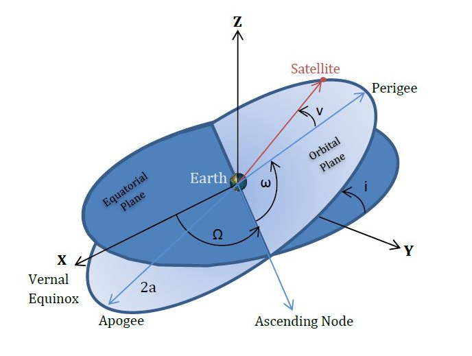
These group into three logical subsets:

(a, e) determine the size and shape of the orbit: shape of ellipse (e<1), parabola (e=1) or hyperbola (e>1)
(i, \(\Omega\), \(\omega\)) define orientation angles of the orbit with respect to some coordinate system (more about this in a bit)
\(\nu\) the position of the body in the orbit denoted as an angle with respect to the line from peripasis to the central body

Note that only \(a\) has units of distance. Eccentricity is a dimensionless number and the remaining elements (\(i, \omega, \Omega, \nu\)) are all angles. Depending on the context the units of \(a\) may be in world units or in physics units. When a COE for an active body in GE is retrieved with ge.COE() it will be in world units.

There are some alternatives to specifying the shape of the orbit which are closely related to the COE and are in some ways more intuitive:

for ellipses the radius at periapsis and apoapsis may be used and then be used to derive the values for a and e
for a hyperbola the periapsis can be used in addition to eccentricity (since the orbit goes to infinity there is no apoapsis)
p may be used to set the size. This then determines the value of a (semi-major axis) for a given e.

When referring to the point of closest approach the term used may vary based on the body being orbited. Perigee for the Earth, perilune for the moon, perihelion for the sun etc. In general we will try to use the generic term periapsis but the use of perigee may sneak in from time to time.

Wikipedia’s Orbit Elements has a good overview.

Circular (e=0) and Flat (i=0) Orbits Can be Tricky¶

There are certain cases which are not well described by the COE. These are generally cases in which one of the key parameters in the COE is zero and this leads to some in-determinism in one of the other parameters.

Case 1: Circular orbits (e = 0). In this case the notion of argument of periapsis is not defined since there no point of closest approach since all points in a circle are the same distance from the center. This leads to an additional complication since the phase (true anomaly) of the orbit is defined with respect to the line to the periapsis. In the case of circular orbits GE2 will reference the true anomaly to the X-axis.

As orbits become close to circular the algorithms for determining argp (\(\omega\)) and true anomaly (\(\nu\)) can be subject to precision issues. Consider an elliptical orbit with the closest approach to the center directly on the y-axis. The orbit phase/true anomaly will be measured from the line from the center to periapsis. A satellite on the y-axis will have a phase \(\nu=0\). If this elliptical orbit gradually becomes circular, then for a circular orbit the position of a ship on the y-axis will have \(\nu=90\) degrees since for a circular orbit the phase reference is the x axis. An algorithm that determines COE from the ship \((r,v)\) state could report \((\omega=90, \nu=0)\) for an orbit slightly above it “circularity threshold” and \((\omega=0, \nu=90)\) if it’s slightly below the orbit threshold. Further, if the orbit is very near this threshold it could dither back forth due to numerical variations as the orbit evolves.

Since Earth satellite orbits are often near-circular this is not simply an oddball edge-case. The best approach in this scenario is to use a new parameter named the argument of latitude: \(u = \omega + \nu\).

Case 2: Flat orbits \((i = 0, i = 180)\) An orbit in the XY plane does not have a line of nodes and therefore \(\Omega\) is not defined. In analogy to the \(e=0\) case above there is parameter longitude of periapsis \(\bar{\omega} = \Omega + \omega\) that can be used when orbits are nearly flat.

How does GE2 handle these cases? When converting an \((r, v)\) state into orbit elements the routine provides an optional parameter small to define how small a parameter needs to be to be considered zero by the algorithm. The default is 1E-6 The API is:

    /// <summary>
    /// Given state information (r,v) and mu=GM determine the classical
    /// orbital elements (COE).
    ///
    /// Classical orbital elements have inherent singularities for:
    /// circular orbits (e=0)
    /// flat orbits (i=0 or Pi radians)
    ///
    /// In this case the sense of how small is zero is set by the optional parameter `small`.
    ///
    /// In the case of circular orbits there is no closest approach point from which to measure phase nu.
    /// For circular orbits the X-axis defines nu=0.
    ///
    /// In the case of a flat orbit, there is no ascending node to provide a reference for omegaU.
    /// It is set to zero.
    ///
    /// See the discussion in the Orbits section of the documentation for other information.
    /// 
    /// </summary>
    /// <param name="r"></param>
    /// <param name="v"></param>
    /// <param name="mu"></param>
    /// <returns></returns>
    public static COE RVtoCOE(double3 r,
                        double3 v,
                        double mu,
                        double small = 1e-6)

The following table shows the behavior of the algorithm. Circular is true if \(e < small\) and flat is true if the orbit is within “small” of 0 or 180 degrees.

Circular	Flat	\(\Omega\)	\(\omega\)	\(\nu\)
yes	no	\(\Omega\)	0	angle from line of node (\Omega)
yes	yes	0	0	angle from x-axis
no	no	\(\Omega\)	\(\omega\)	angle from periapsis
no	yes	0	\(\omega\)	angle from periapsis

Representing COE in GE2¶

The class Orbital.COE represents a set of orbital elements in GE2. The member variables corresponding to the 6 standard values are a, e, i, omegaU, omegaL and nu. Internally, all the angular variables are represented in radians. There are convenience constructors to allow initialization using angles in degrees.

In-scene GSBody objects can specify their initial state using one of several variations of classical orbit elements and designate the body they are in orbit around. See GSBody-Orbits.

The Orbital class in GE2 has the definition of the COE class and several constructors:

   public void EllipseInit(double mu, double a, double e, double i, double omegaL, double omegaU, double nu)
   public void EllipseInitDegrees(double mu, double a, double e, double i, double omegaL, double omegaU, double nu)
   public COE(double mu, double p, double e, double i=0.0, double omegaL=0.0, double omegaU=0.0, double nu=0.0)

Note that in the COE constructor the parameter p is not the periapsis but an size element that is common to ellipses and hyperbolas known as the semi-parameter. It is related to the size element \(a\) by \(p=a(1-e^2)\).

A COE may also be determined from the current \((r,v)\) state using Orbital.RVtoCOE.

Conversely, the \((r, v)\) for an object defined by a COE can be determined with Orbital.COEtoRVRelative.

Generally code using GE2 will make use of the COE class. This is not to be confused with the COEStruct which is needed to pass COE information into the job system. The job system can only make reference to predefined types and not to classes, hence the need for a struct “shadow object”.

Points within an Orbit¶

As shown in the COE Picture there are specific points on an orbit that are of interest:

closest approach (PERIAPSIS)
farthest point (APOAPSIS)
points crossing the equatorial plane (ascending and descending)
points at a specific distance (two per orbit)

These points are defined for a general (non-circular, inclined) orbit. In some cases they may not “make sense” e.g. a circular orbit has no closest or farthest point.

The Orbital class in GE2 has utilities to determine the location of these points of interest in an orbit described by a COE.

Position at time or phase¶

Visualizing Orbits: XY vs XZ¶

By convention all of the mathematical machinery of orbital mechanics takes place in a right-handed coordinate system. All the diagrams in textbooks and online will assume this coordinate system. Unity (and some other graphics systems) uses a left-handed coordinate system. If we take the orbit evolution equations from a physics textbook and render them “as-is” in a Unity scene the orbits will look weird:

satellites will orbit clockwise (vs counter-clockwise according to the usual RH illustrations )
an inclined orbit will have the ascending and descending nodes swapped

This is illustrated explicitly in the sample scene: RightHandedvsLeftDisplay.

[pic here]

GE2 handles this as follows:

in world and physics space everything is aligned with the orbital mechanics textbooks. An orbit with \(i=0\) will be in the XY plane.
GSDisplay allows the user to select XZ orbit mode. In this case an orbit \(i=0\) will be in the XZ plane and the normal will be in the +Y direction. This will make the orbit “look right” (this is done in the MapToScene method).

This is generally ok. The only catch is that applications which make use of transform positions of objects in the display space will need to flip Y and Z values if they want to convert positions to world space. As a general rule it is better to get these values from the GE for the indicated body and avoid referencing the scene positions.

Gravity Engine 2 v3.0

Orbits

Contents